Note
This software has been developed by Stathis Kamperis with major contributions from Chionia Kodona.
Important
This is a work in progress. It is intended for research purposes only.
Table of contents
Use case examples
rteval streamlines the extraction of useful radiotherapy plan parameters from
DICOM data files (RTDOSE, RTPLAN, RTSTRUCT), such as point dose statistics, clinical
dose constraints, arbitrary dose-volume data, contour coordinates, etc. It is easily
scriptable and allows for the analysis of one’s department plans. Either on an
individual plan basis or as a whole.
Its syntax is evolving and currently looks like this:
% python -m rteval.main
Syntax: rteval.py load <RD file> <subcommand>
Available subcommands: ['anonymize', 'beams', 'by', 'cn', 'complexity', 'constraints',
'contour', 'diff', 'dv', 'dvh', 'pointds', 'prescription', 'structs', 'tags', 'vd', 'volume']
%
Each subcommand has its own syntax, e.g.:
% python -m rteval.main load ./443-18/RD.dcm volume
Syntax: volume <structure 1> <structure 2> ...
{"volume": ""}
%
When a structure name is required, it may be given as a regular expression. E.g. To get a list of plan’s structure set:
% python -m rteval.main load ./443-18/RD.dcm structs .*
{"structs": ["BODY", "Cochlea R PRV", "Cochlea R", "Cochlea L PRV", "Cochlea L",
"Brainstem PRV", "Brainstem", "Brain", "Area 51", "CTV 6996", "CTV 5445", "CTV 5940",
"CTV 6600", "CTV Nasal", "Lens R", "CTV Nasopharynx", "Esophagus", "Optic Chiasm PRV",
"Optic Nerv L", "Optic Nerv L PRV", "Optic Nerv R", "Optic Nerv R PRV", "Oral Cavity",
"Parotid L", "Parotid R", "PTV 5445", "oldPTV 5940", "oldPTV 6600", "PTV 6996",
"PTV LN L", "Eye L", "Eye R", "GTV N", "GTV T MRI inbra1", "GTV T MRI inbrai",
"GTV T PET", "CTV LN L", "CTV LN R", "CTV N", "Larynx", "Lens L", "Lens L PRV",
"Lens R PRV", "Optic Chiasm", "PTV LN R", "SMG L", "SMG R", "Spine", "Spine PRV",
"Trachea", "Bolus", "PTV 6600 New", "PTV 5445 New", "PTV 5940 New", "PTV 6303 New",
"PTV patch", "NS_NormalTissue", "Patch", "PTV 5940", "PTV 6600", "PTV 6303",
"PTV1-2", "PTV3-4", "PTV2-3", "PTV4-5"]}
%
To get a list of all structures containing the string “ctv”:
% python -m rteval.main load ./443-18/RD.dcm structs ctv
{"structs": ["CTV 6996", "CTV 5445", "CTV 5940", "CTV 6600", "CTV Nasal",
"CTV Nasopharynx", "CTV LN L", "CTV LN R", "CTV N"]}
%
To get a list of all structures containing the string ‘parotid’ or the string ‘smg’:
% python -m rteval.main load ./443-18/RD.dcm structs 'parotid|smg'
{"structs": ["Parotid L", "Parotid R", "SMG L", "SMG R"]}
%
Get the volume of some structures:
% python -m rteval.main load ./443-18/RD.dcm volume 'parotid|trachea|esophagus|body'
{"volume": {"BODY": "12906.58", "esophagus": "13.11", "parotid_l": "35.22",
"parotid_r": "31.48", "trachea": "31.47"}}
%
Dose constraints report for organs at risk
The following invocation will list all the organs at risk and the values of the respective
constraints. The output is in JSON format and the structure names are fixed regardless of
their original names in the structure set. This is done in order to facilitate subsequent
statistical processing. Hence, Parotid R, R Parotid, Parotid Right, Right Parotid,
Parotid_R, R_Parotid will all become parotid_r.
The nice thing about this feature is that it discovers automatically all known (to rteval) dose constraints:
% python -m rteval.main load ./443-18/RD.dcm constraints
{"constraints": {"brainstem": {"Max": "50.36"}, "cochlea_l": {"Mean": "26.78"},
"cochlea_r": {"Mean": "32.67"}, "esophagus": {"V35": "62.57", "V50": "13.91",
"V70": "0.00", "Mean": "35.79"}, "eye_l": {"Mean": "18.31", "Max": "39.15"},
"eye_r": {"Mean": "20.53", "Max": "42.88"}, "larynx": {"Mean": "41.51"}, "lens_l":
{"Max": "11.10"}, "lens_r": {"Max": "11.58"}, "optic_chiasm": {"Max": "47.10"},
"optic_nerv_l": {"Max": "51.11"}, "optic_nerv_r": {"Max": "51.70"}, "oral_cavity":
{"Mean": "32.61"}, "parotid_l": {"Mean": "45.30"}, "parotid_r": {"Mean": "24.94"},
"smg_l": {"Mean": "64.44"}, "smg_r": {"Mean": "51.19"}, "spine": {"Max": "42.46"},
"trachea": {"Mean": "37.43"}}}
%
Or, in pretty print format:
{
  "constraints": {
      "brainstem": {
          "Max": "50.36"
      },
      "cochlea_l": {
          "Mean": "26.78"
      },
      "cochlea_r": {
          "Mean": "32.67"
      },
      "esophagus": {
          "Mean": "35.79",
          "V35": "62.57",
          "V50": "13.91",
          "V70": "0.00"
      },
      "eye_l": {
          "Max": "39.15",
          "Mean": "18.31"
      },
      ...
  }
Use categorical variables to group results
In many cases one wants to group some measured quantity based on a categorical variable, e.g. measure homogeneity index or conformation number and group the results by the dosimetrist that did the planning or the physician that did the contouring/prescription. This is done by the by subcommand:
% python -m rteval.main load ./443-18/RD.dcm by
Available by clauses: ['operator', 'patient', 'patientID', 'physician', 'plan',
'reviewer', 'studyDate', 'studyDay']
%
For instance, the following command will calculate the conformation number for the
95% isodose of the prescribed dose and attach to the results the reviewer and the
physician:
% python -m rteval.main load ./1010-16/RD.1.2.246.352.71.7.510151505849.233655.20160721142230.dcm \
> by reviewer physician cn auto
{"by": {"reviewer": "maria^papadopoulou", "physician": "kamperis^efstathios"},
        "cn": {"95.0": "0.617"}}
%
The by subcommand is of great value when evaluating many plans at once.
Batch process of plans
Since rteval is merely a Python script, applying it to a set of plans is straightforward.
For instance, the following shell command will list the leaf aperture complexities for all
arcs for all plans in the ~/plan-files directory:
% for f in ~/plan-files/*/RD*.dcm; do python -m rteval.main load "$f" by patientID complexity; done
{"by": {"patientID": "101-16"}, "complexity": {"arc1": "0.642", "arc2": "0.702"}},
{"by": {"patientID": "332-17"}, "complexity": {"arc1": "0.501", "arc2": "0.562"}},
{"by": {"patientID": "443-18"}, "complexity": {"arc1": "0.674", "arc2": "0.626"}},
{"by": {"patientID": "762-17"}, "complexity": {"arc1": "0.556", "arc2": "0.820"}}
Point dose statistics
To print point dose statistics for all structures along with a header for each column:
% python -m rteval.main load ./443-18/RD.dcm pointds header all
Structure            Min   Max   Mean  D2    D98
body                 00.00 76.19 17.54 65.39 00.21
brainstem_prv        18.67 55.11 34.44 50.46 21.10
brainstem            19.90 50.36 33.98 48.12 22.00
brain                00.69 63.80 13.75 47.82 00.96
cochlea_r_prv        28.06 44.25 33.64 41.46 28.91
cochlea_r            29.97 35.68 32.67 35.17 30.55
cochlea_l_prv        23.29 43.04 28.19 38.17 24.10
cochlea_l            24.99 29.93 26.78 29.10 25.23
ctv_6996             62.35 76.19 73.67 75.41 71.21
ctv_5445             04.34 76.19 61.73 74.60 49.92
ctv_5940             04.34 76.19 63.92 74.73 47.13
ctv_6600             57.18 76.19 72.67 75.39 62.07
esophagus            06.22 56.87 35.79 55.03 07.65
eye_l                08.95 39.15 18.31 32.73 09.40
eye_r                08.62 42.88 20.53 35.63 09.55
...
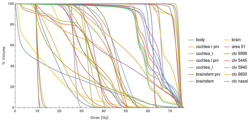
Export DVH data
To export dose-volume data in (dose bin, volume) pairs
you would invoke the dvh subcommand with the paired argument.
The regular expression .* matches all the plan’s structures:
% python -m rteval.main load ./443-18/RD.dcm dvh paired '.*' > dvh.data
%
These data could, then, be plotted with e.g. Mathematica:
jd = Import["dvh.data", "JSON"];
organs = jd[[All, 2, All, 1]][[1]];
getDVH[organ_] := jd[[All, 2, organ, 2, 1(*dv*), 2]][[1]]
ListPlot[ParallelTable[getDVH@k, {k, 1, Length@organs}], Joined -> True,
    InterpolationOrder -> 1, Frame -> {True, True, False, False},
    FrameLabel -> {"Dose [Gy]", "% Volume"}, PlotLegends ->
    Table[organs[[k]], {k, 1, Length@organs}], PlotRangePadding -> {0, 0}]
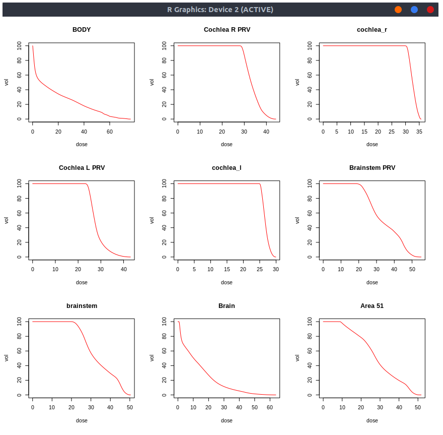
Depending on the software you will be using to process the dvh data,
it may be easier to export all dose bins separately from volume data.
I.e., to export them as [d1, d2, d3, ...], [v1, v2, v3, ...] instead of
[(d1, v1), (d2, v2), (d3, v3), ...]. If this is the case you’d use:
% python -m rteval.main load ./443-18/RD.dcm dvh '.*' > dvh.data
%
And then plot them with R like:
library(jsonlite)
jd <- jsonlite::read_json('dvh.data', flatten=T)
f <- function(organ) {
    df <- data.frame(
        unlist(jd$dvh[[organ]]$dose),
        unlist(jd$dvh[[organ]]$vol)
    );
    names(df) <- c('dose', 'vol');
    return(df)
}
par(mfrow=c(3,3))
for (i in 1:9) { plot(f(i), type='l', col='red', main=organs[[i]]) }
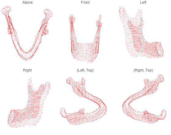
Export contour coordinates
In order to export the coordinates of the points defining a structure, say mandible:
% python -m rteval.main load ./332-17/RD.dcm contour Mandible > mandible.coords
Then you could do whatever you’d feel like with them, e.g. plot them in 3D space
with Mathematica:
struct = Import["~/git-repos/rteval/rteval/mandible.coords", "JSON"]
struct = Flatten[struct[[All, 2, 1, 2]], 1]
Grid[Partition[#, 3] &@
   (ListPointPlot3D[struct, PlotLabel -> #, Axes -> False,
           AspectRatio -> Full, PlotStyle -> {Red}, Ticks -> None,
           Boxed -> False, ViewPoint -> #] & /@
           {Above, Front, Left, Right, {Left, Top}, {Right, Top}})]
Compare two plans against each other
rteval enables the comparison of two plans. The syntax is the following:
% python -m rteval.main load ./443-18/RD.dcm diff
Syntax: load <file 1> diff <file 2> [pretty]
%
So the if we’d like to compare plan 443-18/RD.dcm with 332-17/RD.dcm we’d write:
% python -m rteval.main load ./443-18/RD.dcm diff ./332-17/RD.dcm pretty
Structure       Constr    V1     V2     dV     %
esophagus       V35     62.57  57.18  -5.39  -8.61
esophagus       V50     13.91  18.93   5.02  36.09
esophagus       V70      0.00   0.00   0.00   0.00
esophagus       Mean    35.79  34.49  -1.30  -3.63
larynx          Mean    41.51  41.18  -0.33  -0.79
parotid_l       Mean    45.30  24.41 -20.89 -46.11
parotid_r       Mean    24.94  23.99  -0.95  -3.81
spine           Max     42.46  41.37  -1.09  -2.57
trachea         Mean    37.43  33.56  -3.87 -10.34
%
The optional argument pretty determines whether the output shall be
in plain text columnar format or in JSON format. The comparison includes
only differences in dose constraints, but in the future it will contain
virtually all metrics that rteval can calculate.
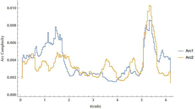
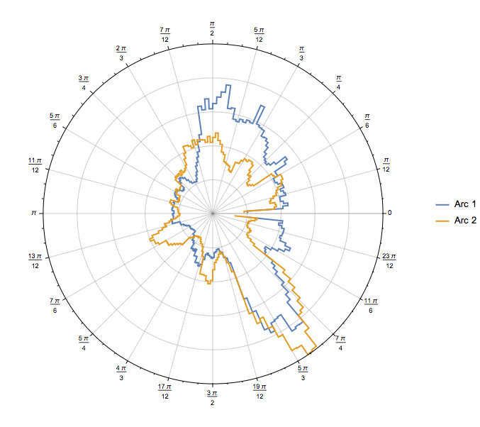
Calculate and visualize the complexities of beam arcs
rteval can calculate the complexity of a plan for every beam
and also it may report the individual “complexities” at each control
point:
% python -m rteval.main load ./443-18/RD.dcm complexity simple
{"complexity": {"simple": {"arc1": "0.674", "arc2": "0.626"}}},
% python -m rteval.main load ./443-18/RD.dcm complexity simple verbose
{"complexity": {"simple": {"arc1": [0.00211, 0.00428, 0.0046, 0.00435, ...]}}}
Then, it’s easy to produce visually appealing plots, like:
json = Import["~/git-repos/rteval/rteval/arcs.json", "JSON"];
arc1 = json[[All, 2, 1, 2, 1, 2]]
arc2 = json[[All, 2, 1, 2, 2, 2]]
dat1 = Table[{2 k Pi/180, arc1[[k]]}, {k, 1, Length@arc1}];
dat2 = Table[{2 k Pi/180, arc2[[k]]}, {k, 1, Length@arc2}];
ListPlot[{arc1, arc2}, Joined -> True, InterpolationOrder -> 0,
    Frame -> {True, True, False, False}, FrameLabel -> {"Theta(rads)", "Arc Complexity"},
    PlotRange -> All, PlotLegends -> {"Arc1", "Arc2"}, ImageSize -> 600]
Or, a polar plot:
Classes
rteval
anonymize
- class anonymize.DicomAnonymizer(dicom_file_path: str)
A class for anonymizing DICOM files. To list the DICOM tags that are anonymized you can call the
list_anonymizable_dicom_tags()static method.>>> from rteval.anonymize import DicomAnonymizer as da >>> da.list_anonymizable_dicom_tags() ['AccessionNumber', 'AdditionalPatientHistory', 'DeviceSerialNumber', 'EthnicGroup', 'InstanceCreationDate', 'InstanceCreationTime', 'Manufacturer', 'ManufacturersModelName', 'NameofPhysiciansReadingStudy', 'OperatorsName', 'OtherPatientIDs', 'OtherPatientNames', 'PatientID', 'PatientAddress', 'PatientAge', 'PatientBirthDate', 'PatientName', 'PatientSex', 'PatientWeight', 'PatientSize', 'PhysiciansofRecord', 'ReferringPhysiciansName', 'ReviewDate', 'ReviewTime', 'ReviewerName', 'SoftwareVersions', 'StationName', 'StudyDate', 'StudyID', 'StudyTime']
- assert_anonymization() None
Confirms that the DICOM file was indeed anonymized, by iterating over all dicom tags and checking that their values were erased as intended. This function is called always by the
do_anonymization()method.
- do_anonymization() None
Performs the anonymization of the respective DICOM file. The result is written to a new file named after the old one plus the suffix
_anon. E.g., given a filefoo.dcm, its anonymized version is saved asfoo.dcm_anon.
- static list_anonymizable_dicom_tags() List[str]
Lists all DICOM tags that this anonymizer can erase. E.g.: PatientID, PatientAddress, PatientAge, etc.
cbct
- class cbct.CBCT(dicom_file_path: str)
A class for discovering Varian CBCT files and assembling them into the right series ordered by their z- coordinate. This is NOT a robust generic class. It serves the purposes of my PhD Thesis.
- check_if_in_order() None
Prints a grid with the CBCT images of the ‘first’ (any, really) CBCT series.
- scan_directory() Dict[str, List[Tuple[str, float]]]
Scan directory for Varian CBCT dicom files and assemble them into the respective series with correct z ordering.
cmd_processor
- class rteval.cmd_processor.CmdProcessor(plan)
This is a class to process the commands that the user enters.
- filter_structs(args: List[str]) List[str]
It treats
argsa regular expression against which matches the structures of the structure set.- Parameters:
args[0] – A regular expression matching structures, e.g.
'.*'to match all structures in the structure set.
If
argsis empty,[]is returned.
- process_anonymize_dicom_file() None
Anonymizes the RD dicom file.
- process_beams(args: List[str]) Dict[str, Any]
- process_by(args: List[str]) Dict[str, Any]
Syntax: … by <clauses> E.g.
>>> python -m rteval.main load /path/to/rd_file cn 'PTV 6996' 95 by reviewer studydate
Will print the conformation number of structure
PTV 6996and will attach the reviewer of the plan and the date it was created to the result.
- process_cn(args: List) Dict[str, Dict[str, str]]
Syntax:
cn <structure regexp> <ref isodose 1> <ref isodose 2> ...Syntax:cn auto
- process_complexity(args: List[str]) Dict[str, Any]
It will return the complexity scores for each beam in the plan.
- Parameters:
Metric – Which complexity metric to calculate.
Verbose – If set, the complexity scores calculated at each control point will be returned.
Differential – The difference of complexity between consecutive control points will be returned.
- process_constraints(arg: List[str], is_reg_exp: bool = True) Dict[str, Dict[str, str]]
Given a regular expression matching structure(s) in the structure set, print their dose constraints.
- Parameters:
arg[0] – If
is_reg_expset toTrue, then this is to be interpreted as a regular expression matching structures, e.g.'.*'to match all structures in the structure set. If set toFalsethenarg[0]is treated as a list of structure names.
E.g.:
>>> from rteval import plan
>>> p = plan.EVPlan('/path/to/rd_file')
>>> p.cmd_processor.process_constraints('paro', is_reg_exp=True)
{'parotid_l': {'Mean': '45.30'}, 'parotid_r': {'Mean': '24.94'}}
>>> e.cmd_processor.process_constraints(
        ['Parotid L', 'Parotid R', 'Spine'], is_reg_exp=False)
{'parotid_l': {'Mean': '45.30'}, 'parotid_r': {'Mean': '24.94'},
    'spine': {'Max': '42.46'}}
- process_contour(args)
Given a regular expression matching structure(s) in the structure set, print the contour coordinates for every CT slice.
- Parameters:
args[0] – A regular expression matching structures, e.g.
'.*'to match all structures in the structure set.
- process_dose_volume(args)
Given a regular expression matching structure(s) in the structure set, print the dose that covers at least
<vol 1> <vol 2> ....- Parameters:
args[0] – A regular expression matching structures, e.g.
'.*'to match all structures in the structure set.args[1 – ]: The list of volume percentages.
E.g.:
>>> from rteval import plan
>>> p = plan.EVPlan('/path/to/rd_file')
>>> p.cmd_processor.process_dose_volume(['paro', 50])
{'parotid_l': {50: '42.57'}, 'parotid_r': {50: '18.50'}}
- process_dump_dose() str
This function retrieves the dose values from the RD file, scales them according to the
DoseGridScalingfactor, and then returns the resulting dose distribution as a pretty-printed JSON string to the standard output.
- process_dvh_data(args)
Given a regular expression matching structure(s) in the structure set, print their dose-volume data.
- Parameters:
paired – If
pairedis set, the return object will be of the form[(d1, v1), (d2, v2), ...]. Otherwise, it will be of the form[(d1, d2, ...), (v1, v2, ...)].
- process_ear(args)
Given a regular expression matching structure(s) in the structure set print the EARs (Excessive Absoulte Risk values) in Grays for the respective structure(s).
- Parameters:
args[0] – The mathematical model to use when estimating OED. Valid values include
linear,expandfrac, for linear, exponential and exponential with fractionation model, respectively.args[1] – A regular expression matching structures, e.g.
'.*'to match all structures in the structure set.args[2] – Age at exposure.
args[3] – Age attained.
- process_list_ct(args: List[str]) Dict[str, str] | None
Print the UIDs of the CT files associated with this plan.
- Parameters:
args[0] – If set to
pretty, the result will be printed in columnar format, rather than in JSON.
- process_list_matching_rules() None
Print the matching rules for structures. Example output: ‘spine matched by: cord spinal_canal spinal_cord spinalcanal spinalcord …’
- process_ntcp(args: List[str]) Dict[str, str]
Given a regular expression matching structure(s) in the structure set, print their normal tissue complication probability (if applicable).
- Parameters:
args[0] – A regular expression matching those structures whose NTCP we would like to calculate. E.g., ‘paro’ will match both ‘Parotid R’ and ‘Parotid L’.
- E.g.:
>>> from rteval import plan
>>> p = plan.EVPlan('/path/to/rd_file')
>>> p.cmd_processor.process_ntcp(['paro'])
    {'parotid_l': '53.66', 'parotid_r': '1.12'}
- process_oed(args)
Given a regular expression matching structure(s) in the structure set print the OEDs (Organ Equivalent Dose values) in Grays for the respective structure(s).
- Parameters:
args[0] – The mathematical model to use when estimating OED. Possible values include
linear,expandfrac, for linear, exponential and exponential with fractionation model, respectively.args[1] – A regular expression matching structures, e.g.
'.*'to match all structures in the structure set.
- process_ovh(args)
Given a regular expression matching structure(s) in the structure set and a structure representing the tumor volume, print the distance of every voxel of every structure to the tumor volume.
- Parameters:
args[0] – A regular expression matching structures, e.g.
'.*'to match all structures in the structure set.args[1] – The structure representing the tumor, e.g.
PTV 5940.args[2] – The grid size, e.g.
100will create a 100x100x100 grid.
- process_plan_diff(args: List[str]) Dict[str, Dict[str, str]]
Print the differences in constraints for two plans.
- Parameters:
args[0] – The second plan to be used in the comparison (the first is the one we have already loaded).
args[1] – If set to
pretty, the result will be printed in columnar format, rather than in JSON.
E.g.:
>>> from rteval import plan
>>> p = plan.EVPlan('/path/to/rd_file')
>>> p.cmd_processor.process_plandiff(['/path/to/rd_file', 'pretty'])
Structure       Constr    V1     V2     dV     %
brainstem       Max     50.38  50.38   0.00   0.00
cochlea_l       Mean    26.78  26.78   0.00   0.00
- process_point_dose_statistics(args: List[str]) Dict[str, Dict[str, str]]
Given a regular expression matching structure(s) in the structure set, print their point dose statistics (Min, Max, Mean, D2, D98).
- Parameters:
args[0] – A regular expression matching structures, e.g.
'.*'to match all structures in the structure set.
E.g.:
>>> from rteval import plan
>>> p = rteval.EVPlan('/path/to/rd_file')
>>> p.cmd_processor.process_point_dose_statistics(['spine'])
{'spine': {'Min': '2.50', 'Max': '42.46', 'Mean': '31.38',
    'D2': '40.37', 'D98': '3.05'},
'Spine PRV': {'Min': '2.05', 'Max': '49.07', 'Mean': '31.22',
    'D2': '44.82', 'D98': '2.54'}}
- process_prescription() Dict[str, float]
Prints the prescription dose of the plan.
- process_software_versions() Dict[str, str]
Prints the Software Versions.
- process_structures(args: List[str]) List[str]
Given a regular expression, print all matching structure(s) in the structure set.
- Parameters:
args[0] – A regular expression matching structures, e.g.
'.*'to match all structures in the structure set.
E.g.:
>>> from rteval import plan
>>> p = plan.EVPlan('/path/to/rd_file')
>>> p.cmd_processor.process_structures(['paro'])
['Parotid L', 'Parotid R']
- process_tags(arg: List[str]) str
Prints DICOM tags in RTDOSE, RTPLAN or RTSTRUCT files.
- Parameters:
arg[0] – One of the values:
rd,rporrs.
- process_total_mus() Dict[str, str]
Print the total number of monitor units for all beams.
- process_volume_dose(args: List[str | int]) Dict[str, Dict[int, str]]
Given a regular expression matching structure(s) in the structure set, print the volume that receives at least
<isodose 1> <isodose 2> ....- Parameters:
args[0] – A regular expression matching structures, e.g.
'.*'to match all structures in the structure set.args[1 – ]: A list with isodoses.
E.g.:
>>> from rteval import plan
>>> p = plan.EVPlan('/path/to/rd_file')
>>> p.cmd_processor.process_volume_dose(['paro', 30, 50])
{'Parotid L': {30: '34.04', 50: '21.73'}, 'Parotid R': {30: '13.85', 50: '7.91'}}
- process_volume_of_structure(args: List[Any]) Dict[str, str]
Given a regular expression matching structure(s) in the structure set, print the volume of each one of them.
- Parameters:
args[0] – A regular expression matching structures, e.g.
'.*'to match all structures in the structure set.
E.g.:
>>> from rteval import plan
>>> p = plan.EVPlan('/path/to/rd_file')
>>> p.cmd_processor.process_volume_of_structure(['paro'])
{'parotid_l': '35.22', 'parotid_r': '31.48'}
complexity
- class complexity.Complexity(rtplan: Dataset, beam: Dataset)
- calc_area(aleafs: list[float], bleafs: list[float]) float
Calculates the area defined by the leafs.
- calc_complexity() tuple[float, list[float]]
Calculates the complexity for this beam.
- Returns:
A tuple
(x, y), wherexis the total complexity for this beam andyis a list with the complexities of each individual CP.
- calc_complexity_at_cp(cp: int) float
- calc_differential_complexity() tuple[float, list[float]]
Calculates the differential of complexity for this beam.
\[\text{Differential} = \left|\text{Complexity}_{i+1} - \text{Complexity}_{i}\right|\]For all \(i\).
- Returns:
A tuple
(x, y), wherexis the total differential complexity for this beam andyis a list with the differential complexities of each individual CP.
- calc_leaf_end_perimeter(aleafs: List[float], bleafs: List[float]) float
Calculates the perimeter of the area defined by the leafs.
- calc_leaf_side_perimeter(aleafs: List[float], bleafs: List[float]) float
Calculates the perimeter of the leaf sides only. I.e., it does not include the perimeter due to leafs width.
- get_complexity_metric(metric_name: str) Any
- get_jaw_leaf_pos(cp: int) Tuple[Dict[str, List[float]], List[float], List[float]]
Returns the leaf positions for the
cpcontrol point.Note:
[0x300a, 0x11c]is the Leaf/Jaw Positions attribute.
- get_leaf_width(leaf: int) int
Returns the leaf width for
leafin millimeters.In some linacs the leaf width is smaller at the center. E.g. in Varian Clinac DHX, the collimator has 120 MLC (field size 40x40 cm), central 20 cm of field - 5mm leaf width, outer 20 cm of field - 10 mm leaf width.
- get_monitor_units() list[float]
Returns a list with the number of monitor units for every control point. E.g. [0, 2.45, 2.60, 2.60, 2.53, 1.63, 1.54, 1.20, …]
The MUs are calculated via the following formula: MU = meterset weight * beam meterset / final cumulative meterset weight
- get_number_of_leafs() int
Returns the number of leafs.
In Varian Clinac DHX the collimator has 120 leafs.
- get_total_monitor_units() float
Returns the total number of Monitor Units for this beam.
- jaws_block_leafs(cp: int) bool
Check if jaws block leafs of the MLC collimator.
- Parameters:
cp (int) – The number of control point to check.
- Returns:
True, if the jaws block the leafs, orFalseotherwise.
constraints
- class rteval.constraints.Constraint(structure: str, differential_dvh: DVH)
A class for calculating the values of clinical constraints for organs at risk.
The constraints are picked automatically, e.g. if the structure is
Spinal Cordthen automatically maximum point dose is returned. If the structure isLungthen automaticallyMean dose,V5,V13,V20andV30are returned. Which constraint is returned for every organ, is specified in thespec_constraints.pyfile.- Parameters:
structure (str) – The name of the structure, e.g.
Spinal Cord.differential_dvh (mydvh.DVH) – The associated differential Dose-Volume Histogram.
- calc_ear(model: str, prescribed_dose: float, dose_per_fraction: float, agex: float, agea: float) Tuple[float, float, float] | None
Returns the EAR (Excess Absolute Risk) using
model.- Parameters:
model (str) – The model to be used for the calculation. Valid values include
linear,expandfrac.prescribed_dose (int) – The prescribed dose for the treatment.
dose_per_fraction (int) – Dose per fraction.
- calc_max_dose() Tuple[str, float]
Returns the max point dose from the DVH DICOM data.
E.g.:
>>> from rteval.import plan
>>> from rteval.constraints import Constraint
>>> p = plan.EVPlan('/path/to/rd/file)
>>> con = Constraint('Spine', p.get_dvh_of('Spine'))
>>> con.calc_max_dose()
('Max', 42.46000000000012)
- calc_mean_dose() Tuple[str, float]
Returns the mean dose from the DVH DICOM data.
E.g.:
>>> from rteval.import plan
>>> from rteval.constraints import Constraint
>>> p = plan.EVPlan('/path/to/rd/file)
>>> con = Constraint('Parotid R', p.get_dvh_of('Parotid R'))
>>> con.calc_mean_dose()
('Mean', 24.9401782163357)
- calc_ntcp() float | None
Returns the NTCP calculated via the LKB model. If the organ class does not have
get_lkb_parameters()method, returnNone.E.g.:
>>> from rteval.import plan
>>> from rteval.constraints import Constraint
>>> p = plan.EVPlan('/path/to/rd/file)
>>> con = Constraint('Parotid R', p.get_dvh_of('Parotid R'))
>>> con.calc_ntcp()
4.7632661193966594
- calc_oed(model: str, prescribed_dose: float, dose_per_fraction: float) Tuple[float, float, float] | None
Calculates and returns the Organ Equivalent Dose (OED) using the provided model.
- Parameters:
model (str) – The model to be used for the calculation. Valid values include
linear,expandfrac.prescribed_dose (int) – The prescribed dose for the treatment.
dose_per_fraction (int) – Dose per fraction.
- Returns:
The calculated OED value if successful, otherwise
None.- Return type:
float
- calc_v(constraints: List[int]) List[Tuple[str, float]]
Returns Dose Volume constraints.
Constraints are given as a list V_D values. E.g.,
[20, 40, ...]corresponds to(V20, V40, ...). If aDvalue is given that exceeds the global Dmax then0is returned.
- static get_list_of_constraints()
- get_standard_name_of_structure(structure: str) str
Returns the standard name for
structure.Given a structure name, e.g. Right Parotid`, return its standard name, e.g.
parotid_r. If none found, return the normalized version of the argument itself, i.e.,right_parotid. This is useful for aggregating data for later statistical evaluation.
- match_constraint() List[Tuple[str, str, float]]
Returns a list with tuples each tuple corresponding to a matched constraint.
E.g.:
>>> from rteval import plan
>>> from rteval.constraints import Constraint
>>> p = plan.EVPlan('/path/to/rd/file)
>>> Constraint('Larynx', p.get_dvh_of('Larynx')).match_constraint()
    [['larynx', 'Mean', 41.5100257507431]]
- match_organ_class()
Returns the organ class for this structure.
direval
- class direval.DirectoryEvaluator(root_directory, file_tasks)
A class for traversing a directory hierarchy in order to discover RTDOSE dicom files. Once found, the files are processed with
rtevalin parallel.The
find_worker()method will find all RTDOSE dicom files under the root directory. For each one of them it will execute therteval.main()method and it will pass whatever argument was given to us. E.g.:>>> python -m rteval.direval /temp constraints '.*'
Will look for RTDOSE dicom files under
/tempand for each one of them it will call:>>> python -m rteval.main load <file> constraints '.*'
- eval_worker() None
- find_worker(rlist: ListProxy)
- start_eval() None
- direval.direval_main() None
dose_prescription
- class rteval.dose_prescription.DosePrescription(plan: EVPlan, doseref: List[int] | None = None)
A class for inferring dose prescription levels in plans with a simultaneous integrated boost (SIB).
- Parameters:
plan (EVPlan) – The plan whose dose prescription we want to extract.
doseref (list) – A list of predetermined dose levels, likely to be department specific, to which the inferred doses are rounded. If none given then assume
[5280, 5445, 5940, 6600, 6996].
- get_max_prescribed_dose() Tuple[float, str]
This can be retrieved either by
Target Prescription Doseif the prescription was done via a structure with Dose Reference TypeTARGETor byDelivery Maximum Doseif the structure is ofORGAN_AT_RISKtype. The search is done across all beams.- Returns:
A tuple
(x, y)withxbeing the maximum prescribed dose andythe structure from which this dose level was inferred.
- infer_sib_doses() List[Tuple[str, int]]
Use heuristics to infer dose prescription levels in plans with a simultaneous integrated boost (SIB). It may return inaccurate results.
- Returns:
A list of
(x, y)tuples withxbeing some PTV andybeing the inferred dose level (rounded to the closest predetermined dose level).E.g.:
>>> from rteval import plan, dose_prescription as dp
>>> p = plan.EVPlan('/path/to/rd_file)
>>> dp.DosePrescription(p).infer_sib_doses()
[('PTV LN R', 5445), ('PTV 5445 New', 5445), ('PTV LN L', 5445), ('PTV1-2', 5445), ('PTV 5445', 5445), ('PTV 5940', 5940), ('PTV3-4', 5940), ('PTV2-3', 5940), ('PTV 5940 New', 5940), ('oldPTV 5940', 5940), ('PTV 6600', 6600), ('PTV4-5', 6600), ('PTV 6303 New', 6600), ('PTV 6600 New', 6600), ('PTV 6303', 6600), ('oldPTV 6600', 6600), ('PTV 6996', 6996)]
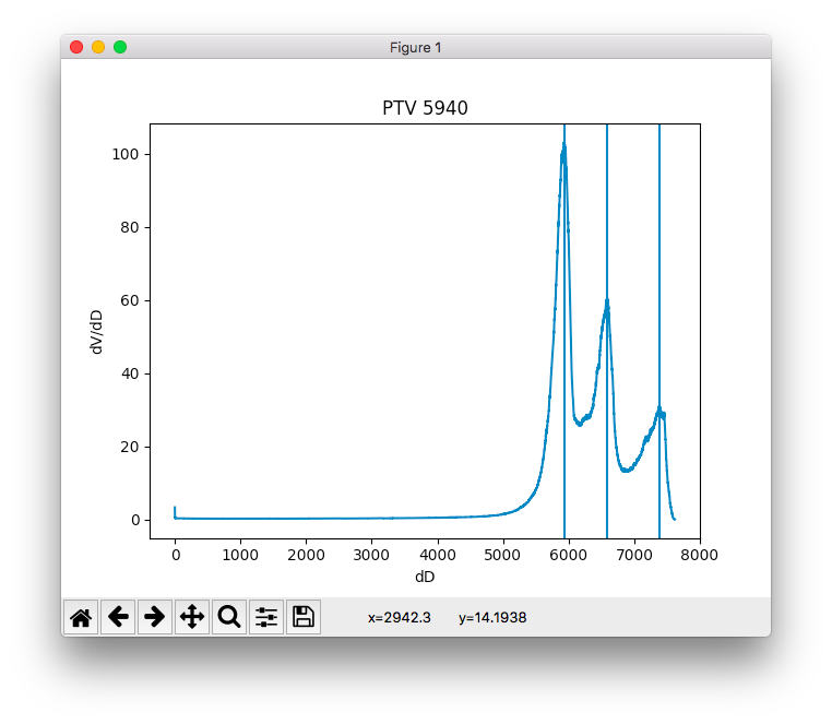
- plotd_dvh_peaks() None
Plot differential DVH along with the detected peaks corresponding to the dose levels (rounded to the closest predetermined dose level).
This method is meant to be used for debugging purposes.
margins
- class rteval.margins.iso3dmargin.Iso3DMargin(coords: List[Tuple[float, float, float]], margin: float)
Example:
>> from rteval.margins import iso3dmargin
>> i3 = iso3dmargin.Iso3DMargin.from_file_path(file_path='./tests/443-18/ptv.coords', structure='PTV 5445', margin=10)
>> i3.plot_it()
- classmethod from_file_path(file_path: str, structure: str, margin: float) Iso3DMargin
Load the vertex coordinates from a file.
- Parameters:
file_path (str) – Path to the file with the vertex coordinates.
structure (str) – The name of the structure to which the margin will be applied, e.g.
spine.margin (float) – The value of the margin to add.
- iso_margin()
Add isotropic margin across the x, y and z axes.
The margin is implemented as the union of a structure dilated across the positive and across the negative of x, y and z axes.
- plot_it() None
Plot the dilated structure.
Useful for debugging purposes.
- class rteval.margins.xymargin.XYMargin(coords: List[Tuple[float, float, float]], margin: float)
- dilate_all_polys() List[List[Tuple[float, float, float]]]
Dilate all polygons in the structure by the margin.
- Returns:
A list of coordinates for all dilated polygons.
- Return type:
List[CoordsType]
- dilate_poly(z0: float) List[Tuple[float, float, float]]
Dilate the polygon at a given z-value by the margin.
- Parameters:
z0 (float) – The z-value of the polygon to dilate.
- Returns:
The coordinates of the dilated polygon.
- Return type:
CoordsType
- filter_z(z0: float) List[Tuple[float, float, float]]
Filter coordinates based on a given z-value.
- Parameters:
z0 (float) – The z-value to filter by.
- Returns:
A list of coordinates that have the given z-value.
- Return type:
CoordsType
- classmethod from_file_path(file_path: str, structure: str, margin: float) XYMargin
Load the vertex coordinates from a file.
- Parameters:
file_path (str) – Path to the file with the vertex coordinates.
structure (str) – The name of the structure to which the margin will be applied, e.g.
spine.margin (float) – The value of the margin to add.
- get_linear_ring(z0: float) shapely.geometry.LinearRing
Create a LinearRing for a given z-value using shapely.geometry.
- Parameters:
z0 (float) – The z-value to filter by.
- Returns:
A LinearRing object.
- Return type:
sg.LinearRing
- get_xy(z0: float) List[Tuple[float, float]]
Get x, y pairs for a given z-value.
- Parameters:
z0 (float) – The z-value to filter by.
- Returns:
A list of (x, y) coordinate pairs.
- Return type:
List[Tuple[float, float]]
- get_zs() List[float]
Get all unique z-values from the coordinates.
- Returns:
A list of unique z-values.
- Return type:
List[float]
- plot_it() None
Plot the dilated structure.
Useful for debugging purposes.
- rteval.margins.xymargin.main() None
mydvh
- class rteval.mydvh.DVH(differential_dvh: Dataset, structure: str, prescribed_dose: float)
This is a wrapper class around the Pydicom DVH class.
- Parameters:
differential_dvh (pydicom.Dataset) – The Pydicom DVH object corresponding to a differential DVH.
structure (str) – The structure this DVH is associated with.
prescribed_dose (float) – The maximum prescribed dose.
- differential_dvh
The Pydicom DVH object.
- Type:
pydicom.Dataset
- structure
The name of the structure associated with this DVH.
- Type:
str
- abs_cumulative() List[float]
Returns the absolute cumulative DVH.
- calc_rel_cumulative() None
Calculates the relative cumulative DVH.
- fast_calc_abs_cumulative() None
Calculates fast the absolute cumulative DVH.
- get_dicom_dvh() Dataset
Returns the Pydicom differential DVH data object.
- get_dose_of_volume(vol_percentage: float) float
Returns the minimum dose that covers
vol_percentageof the structure.E.g., get_dose_colume(95) for ‘PTV’ structure will return the D95 of PTV, i.e. the minimum dose that covers 95% of the PTV volume.
>>> from rteval import plan
>>> p = plan.EVPlan('/path/to/rd_file')
>>> p.get_dvh_of('Brainstem').get_dose_volume(0.01)
50.179999999998586
- get_dvh_data(paired: bool = False) Dict
Returns a dictionary with dose bin and volume data for the structure that is associated with this DVH.
The exact structure of the returned dictionary depends on the value of the parameter
paired.- Parameters:
paired – If set to
Truethen (dose bin, volume) pairs are returned. If set toFalsethen the resultant dictionary will have two nested dictionaries nameddoseandvol, each containing dose bin and volume data, respectively.
With
paired=False:>>> from rteval import plan >>> p = plan.EVPlan('/path/to/rd_file') >>> p.get_dvh_of('Lens L').get_dvh_data(paired=False) {'dose': [0.0, 0.01, 0.02, 0.03, 0.04, ...], 'vol': [100.0, 100.0, 100.0, 99.98, 99.1, ...]}
Same as before but with
paired=True:>>> from rteval import plan >>> p = plan.EVPlan('/path/to/rd_file') >>> p.get_dvh_of('Lens L').get_dvh_data(paired=True) {'dv': [(0.0, 100.0), (0.01, 100.0), (0.02, 100.0), (0.03, 99.98), (0.04, 99.97), ...]}
- get_max_dose(manual: bool = False) float
Returns the max dose for the structure that is associated with this DVH. Normally, the max dose should be available via Pydicom’s
DVHMaximumDose. In case it isn’t, this function can be used to calculate it.E.g.:
>>> from rteval import plan
>>> p = plan.EVPlan('/path/to/rd/file')
>>> p.get_dvh_of('Spine').get_max_dose()
42.46000000000012
- get_mean_dose(manual: bool = False) float
Returns the mean dose for the structure that is associated with this DVH. Normally, the mean dose should be available via Pydicom’s
DVHMeanDose. In case it isn’t, this function can be used to calculate it.The formula that is used is the following:
\[\text{Mean dose} = \frac{1}{\text{Total Volume}} (\mathrm{d}V_1 \mathrm{d}D_1 + \mathrm{d}V_2 \mathrm{d}D_2 + \ldots)\]for all dose bins, \(\mathrm{d}V\), and their respective volume bins, \(\mathrm{d}V\).
- get_min_dose(manual: bool = False) float
Returns the min dose for the structure that is associated with this DVH. Normally, the min dose should be available via Pydicom’s
DVHMinimumDose. In case it isn’t, this function can be used to calculate it.>>> from rteval import plan >>> p = plan.EVPlan('/path/to/rd/file') >>> p.get_dvh_of('CTV 6996').get_min_dose() 62.3490123432927
- get_total_volume() float
Returns the total volume of structure.
NOTE: This function uses the absolute cumulative DVH to retrieve the total volume of the structure.
>>> from rteval import plan
>>> p = plan.EVPlan('/path/to/rd_file')
>>> p.get_dvh_of('Brainstem').get_total_volume()
20.091246543670735
- get_total_volume2() float
Returns the total volume of structure.
NOTE: This function uses the differential DVH to retrieve the total volume of the structure.
>>> from rteval import plan
>>> p = plan.EVPlan('/path/to/rd_file')
>>> p.get_dvh_of('Brainstem').get_total_volume()
20.091246543670735
- get_volume_dose(isodose: int | float) float
Returns the volume that is irradiated with at least
isodoseof the prescribed dose.>>> from rteval import plan >>> p = plan.EVPlan('/path/to/rd_file') >>> p.get_dvh_of('PTV 5940').get_volume_dose(0.5) 721.6103704975708
This is useful for the calculation of conformity index, i.e. CI = PTV / IRVol95.
- rel_cumulative() List[float]
Returns the relative cumulative DVH.
ntcp
- class rteval.ntcp.lkb_model.LKBModel(dvh: DVH, parameters: List[Any])
The Lyman Kutcher Burman (LKB) model is one of the most well known models for predicting Normal Tissue Complication Probability (NTCP) in a radiation treatment plan.
There are three parameters in the LKB model.
TD50represents the dose for a homogenous dose distribution to an organ at which 50% of patients are likely to experience a defined toxicity within 5 years.mis related to the standard deviation of TD50 and describes the steepness of the dose-response curve andnindicates the volume effect of the organ being assessed.- calc_deff(n: float) float
Calculate effective dose deff, i.e. the dose that, if given uniformly to the entire volume, will lead to the same NTCP as the actual non-uniform dose distribution.
- Parameters:
n (float) – The model’s parameter
n.
The model uses the following formula:
\[D_\text{eff} = \sum_{i=1}^{N} (v_i D_i^n)^{1/n}\]Where \(v_i\) is the fractional volume receiving \(D_i\) dose summed over all \(N\) voxels. In a differential DVH the y axis is \(\mathrm{d}V/\mathrm{d}D\), therefore \(v_i = (\mathrm{d}V/\mathrm{d}D) \cdot \mathrm{d}D / V_\text{total}\). X axis is \(\mathrm{d}D\), therefore \(D_i = \sum_j \mathrm{d}D_j\).
- calc_ntcp() float
Calculate the NTCP via the following formula:
\[\text{NTCP} = \frac{1}{2\pi}\int_{-\infty}^t \exp\left( -\frac{t^2}{2}\right)\mathrm{d}t\]Where:
\[t = \frac{D_\text{eff} - \text{TD}_{50}}{m \text{TD}_{50}}\]
- class rteval.ntcp.ntcp_calculator.NTCPCalculator(dvh: DVH, parameters: List[Any])
A class for calculating Normal Tissue Complication Probabilities (NTCPs).
- Parameters:
dvh (mydvh.DVH) – A differential DVH object.
parameters (list) – A list of values, with the first element corresponding to the mathematical model to use when estimating NTCP. Possible values currently only include
LKB.
- calc_ntcp() float | None
Do the actual calculation of NTCP.
oed
- class rteval.oed.oed_calculator.OEDCalculator(dvh: DVH, model: List[Any])
A class for calculating Organ Equivalent Doses (OEDs).
- Parameters:
dvh (mydvh.DVH) – A differential DVH object.
model – The mathematical model to use when estimating OED. Possible values include
linear,expandfrac.
- calc_oed() Tuple[float, float, float] | None
Do the actual calculation of OED.
- rteval.oed.oed_calculator.calc_mu(age_exposure: float, age_attained: float, ge: float, ga: float) float
Calculates the modifying function \(mu\) that contains the population dependent variables.
The \(mu\) function is defined as:
\[\mu(agex, agea) = \exp\left( \gamma_e (agex-30) + \gamma_a \ln \left( \frac{agea}{70}\right) \right)\]Reference: https://www.ncbi.nlm.nih.gov/pmc/articles/PMC3161945/
- Parameters:
agex (float) – Age at exposure
agea (float) – Age attained
ge (float) – Age modifying parameter
ga (float) – Age modifying parameter
- class rteval.oed.linear_model.LinearModel(dvh: DVH, parameters: List[Any])
A Linear model for calculating Organ Equivalent Doses (OEDs) in the context of predicting the risk of secondary (radiation-induced) cancers.
The model uses the following formula:
\[\text{OED} = \sum_{i=1}^{N} v_i D_i\]Where \(v_i\) is the fractional volume receiving \(D_i\) dose summed over all \(N\) voxels. In a differential DVH the y axis is \(\mathrm{d}V/\mathrm{d}D\), therefore \(v_i = (\mathrm{d}V/\mathrm{d}D) \cdot \mathrm{d}D / V_\text{total}\). X axis is \(\mathrm{d}D\), therefore \(D_i = \sum_j \mathrm{d}D_j\).
- Parameters:
dvh (mydvh.DVH) – The associated differential Dose-Volume Histogram.
parameters (list) – The model’s parameters.
- calc_oed() Tuple[float, float, float]
Calculates the OED in Gray (Gy).
- Returns:
The value of OED.
- class rteval.oed.exp_model.ExpModel(dvh: DVH, parameters: List[Any])
An exponential model for calculating Organ Equivalent Doses (OEDs) in the context of predicting the risk of secondary (radiation-induced) cancers.
The model uses the following formula:
\[\text{OED} = \sum_{i=1}^{N} v_i D_i \exp(-\alpha D_i)\]Where \(v_i\) is the fractional volume receiving \(D_i\) dose summed over all \(N\) voxels. In a differential DVH the y axis is \(\mathrm{d}V/\mathrm{d}D\), therefore \(v_i = (\mathrm{d}V/\mathrm{d}D) \cdot \mathrm{d}D / V_\text{total}\). X axis is \(\mathrm{d}D\), therefore \(D_i = \sum_j \mathrm{d}D_j\).
- Parameters:
dvh – The associated differential Dose-Volume Histogram.
parameters – The model’s parameters.
- calc_oed() Tuple[float, float, float]
Calculates the OED in Gray (Gy).
- Returns:
A tuple of the form
(x, y, z)wherexis the calculated OED for a givenalphavalue, andyandzare the lower and upper bounds of OED corresponding to the lower and upper bounds of thealphavalue.
- do_calc_oed(alpha: float) float
Perform the actual OED calculation for a single
alphavalue.- Parameters:
alpha (float) – The model’s parameter alpha.
- Returns:
The value of OED for this particular
alphavalue.
- class rteval.oed.frac_model.FracModel(dvh: DVH, parameters: List[Any])
An exponential model for calculating Organ Equivalent Doses (OEDs) in the context of predicting the risk of secondary (radiation-induced) cancers, that takes into account cell killing and fractionation effects. Reference: https://tbiomed.biomedcentral.com/articles/10.1186/1742-4682-8-27
The model uses the following formula:
\[\text{RED}(D) = \frac{e^{-d D}}{a' R} \left( 1 -2R + R^2 e^{a' D} - (1-R^2) e^{-\frac{a'R}{1-R}D}\right)\]Where it assumed that the tissue is irradiated with a fractionated treatment schedule of equal dose fractions \(d\) up to a dose \(D\). The number of cells is reduced by cell killing which is proportional to \(a'\) and is defined using the linear quadratic model:
\[a' = a + \beta d = a + \beta \frac{D}{D_T} d_T\]Where \(D_T\) and \(d_T\) is the prescribed dose to the target volume with the corresponding fractionation dose, respectively. An \(a/\beta\) ratio of 3 is assumed, with \(a=0.1\) and \(\beta=0.033\).
- Parameters:
dvh – The associated differential Dose-Volume Histogram.
parameters – The model’s parameters.
- RED(prescribed_dose: float, dose_per_fraction: float, R: float, D: float) float
- calc_ear(agex: float, agea: float, ge: float, ga: float) float
Calculates the Excess Absolute Risk (EAR) for a whole organ.
- Parameters:
agex (float) – Age at exposure.
agea (float) – Age attained.
ge (float) – Age modifying parameter.
ga (float) – Age modifying parameter.
- calc_oed() Tuple[float, float, float]
Calculates the OED in Gray (Gy).
- Returns:
OED in Gray (Gy)
- do_calc_oed(prescribed_dose: float, dose_per_fraction: float, R: float) float
Perform the actual OED calculation.
- Parameters:
prescribed_dose (float) – The prescribed total dose, e.g. 70 Gy.
dose_per_fraction (float) – Dose per fraction, e.g. 2 Gy/fraction.
R (float) – Repopulation factor. Must be in [0, 1].
- Returns:
The value of OED.
ovh
- class rteval.ovh.OVH(coords: Dict[str, List[List[float]]], nsize: int)
- Parameters:
coords – the coordinates in R^3 of the structure that will participate in overlap histogram calculation, e.g. ‘Spine’ and ‘PTV 5940’.
nsize – The size of the grid, e.g. nsize=100 will create a 100x100x100 grid.
- calcd_ovh(organ: str, target: str) List[float]
Calculates the differential overlap histogram between
organandtarget.
- classmethod from_file_path(file_path: str, nsize: int)
Load the vertex coordinates from a file.
- Parameters:
file_path – Path to the file with the vertex coordinates.
nsize – The size of the grid, e.g. nsize=100 will create a 100x100x100 grid.
- plot_hist(d_ovh: List[float]) None
Plots
d_ovhdifferential overlap histogram. This is used primarily for debugging purposes.
- write_to_file(d_ovh: List[float], organ: str) None
Writes
d_ovhdifferential overlap histogram fororganin the disk. This is used primarily for debugging purposes.
- rteval.ovh.main() None
plan
- class rteval.plan.EVPlan(rd_file_path: str)
A class representing a radiotherapy RTDOSE file.
The EVPlan class is designed to encapsulate various clinical and dosimetric information extracted from an RTDOSE file. This file is a part of the DICOM standard used in radiotherapy for dose distributions. Beyond just the RTDOSE file, the EVPlan class also associates the related RTPLAN and RTSTRUCT files, allowing for a more comprehensive view of a radiotherapy plan.
- - rd_file_path
Path to the RTDOSE file. This can be a direct path to a DICOM file or a path to a zip file containing the DICOM file.
- Type:
str
- - basepath
The base directory where the RTDOSE file is located. This is used to resolve relative paths to associated RTPLAN and RTSTRUCT files.
- Type:
str
- - rtdose
The loaded RTDOSE DICOM dataset.
- Type:
pydicom.Dataset
- - rtplan
The associated RTPLAN DICOM dataset.
- Type:
pydicom.Dataset
- - rtss
The associated RTSTRUCT DICOM dataset.
- Type:
pydicom.Dataset
- - structure_set
An instance of
StructureSetwhich represents the structures defined in the RTSTRUCT file.
- - cmd_processor
An instance of
CmdProcessorwhich can process commands related to this radiotherapy plan.
E.g.:
>>> from rteval import plan
>>> p = plan.EVPlan('/path/to/rd/file)
>>> p.get_number_of_fractions()
33
>>> p.get_prescribed_dose()
('69.96', 'PTV 6996')
>>> p.structure_set.get_structures()
['BODY', 'Brainstem PRV', 'Brainstem', 'Brain', 'CTV 6996', ..., 'Spine', ...]
- RTDOSE_MOD = 'RTDOSE'
- RTPLAN_MOD = 'RTPLAN'
- RTSTRUCT_MOD = 'RTSTRUCT'
- cleanup(path_to_temp_dir: str) None
- get_beam_sequence() Sequence
Returns the beam sequence of the plan.
- get_complexity(metric_name: str, differential: bool = False, verbose: bool = False) List[Tuple[str, float]] | List[Tuple[str, float, List[float]]]
Returns the complexities for every beam in the plan. The beam names are normalized for easier post-processing.
- Parameters:
metric_name (str) – Complexity metric to calculate. Options: ‘coa’, ‘em’, ‘efs’, ‘ltmean’, ‘mcs’, ‘mcsv’, ‘mfa’, ‘pi’, ‘sas’.
differential (bool) – If True, calculates ‘differential’ complexity.
verbose (bool) – If True, returns individual complexities for each control point of the beams.
- Returns:
List of tuples. If verbose is False: List contains tuples (beam_name, total_complexity). If verbose is True: List contains tuples (beam_name, total_complexity, control_point_complexities).
- get_conformation_number(structure: str, isodose: int | float) float
Returns the conformation number for
structureat the specifiedisodoselevel, as per the van’t Riet et al definition.- Parameters:
structure (str) – The name of the structure, e.g.
PTV 5940.isodose (int) – Isodose level given as a percentage, e.g.
95corresponds to the95%of prescribed dose.
- Returns:
Conformation number ranging in [0.0, 1.0].
- get_dose_constraints(structure: str) List[Tuple[str, str, float]] | None
Returns the dose constraints for
structure(organ at risk).Depending on the structure that is probed, the respective constraints are automatically calculated. E.g., if
argisLungthenV20for lung will be returned, whereas ifargisSpinal Cordspine’s max point dose will be returned.- Parameters:
structure (str) – The name of the structure, e.g.
Lung.- Returns:
A list of [‘Structure’, ‘Constraint’, Numerical value]. E.g., [[‘lung’, ‘V5’, 45], [‘lung’, ‘V20’, 30], [‘lung’, ‘Mean’, 20], …], or
Noneif there are no known dose constraints forstructure.
- get_dose_volume(structure: str, vol_percentage: int | float) float | None
Returns the dose that covers at least
vol_percentageofstructure.- Parameters:
structure (str) – The name of the structure, e.g.
PTV 5940.vol_percentage (int) – Percentage of volume, e.g.
95corresponds to the95%the structure’s total volume.
>>> python -m rteval.main load ./443-18/RD.dcm dv 'PTV 5445' 95
{"dv": {"PTV 5445": {"95.0": "52.45"}}}
>>> python -m rteval.main load ./443-18/RD.dcm dv 'PTV 6600' 95
{"dv": {"PTV 6600": {"95.0": "63.71"}}}
- get_dvh_of(structure: str) DVH | None
Returns the Dose-Volume Histogram (DVH) of
structure.- Parameters:
structure (str) – The name of the structure, e.g.
PTV 5940.- Returns:
The DVH data object if it exists or
Noneotherwise.
- get_ear(model: str, structure: str, agex: float, agea: float) Tuple[float, float, float] | None
Returns the Excessive Absolute Risk for
structure.
- get_input_file_name() str
- get_institution_name() str
Returns the Institution’s Name where where the equipment is located that is to be used for beam delivery.
- get_ntcp(structure: str) float | None
Calculates the normal tissue complication probability (NTCP) for a given structure.
- Parameters:
structure (str) – The name of the structure.
- Returns:
A float representing the NTCP probability or
None.
- get_number_of_beams() Tuple[int, int]
Returns the number of beams in the plan broken down by their type, i.e., static vs. dynamic.
- Returns:
A tuple where the first element is the number of static beams and the second element is the number of dynamic beams in the plan.
- get_number_of_fractions() int
Returns the number of fractions planned.
- get_oed(model: str, structure: str) Tuple[float, float, float] | None
Returns the organ equivalent dose value (if applicable).
- get_operator_name() str
Returns the normalized name of the operator.
The username that was used while logged in (to TPS?).
- get_patient_id() str
Returns the patient’s unique identification number.
- get_patient_name() str
Returns the normalized patient’s name.
- get_physician_name() str
Returns the normalized physician name.
- get_plan_label() str
Returns the normalized RT plan label, e.g.
plan1orplan_nasopharynx.
- get_point_dose_statistics(structure: str) List[Tuple[str, float | None] | None]
Returns a list of (statistic, value) for
structureor an empty list if an error has occured.- Parameters:
structure (str) – The name of the structure, e.g.
PTV 5940.
The statistics include Min point dose, Max point dose, Mean dose, D2 and D98.
- get_prescribed_dose() Tuple[float, str]
Returns the plan’s prescribed dose.
- Returns:
A tuple
(x, y)is returned, withxbeing the prescribed dose andythe structure that is attached to it.
In plans with a simultaneous integrated boost (SIB), returns the highest dose level. So if the patient is treated with 6996/212, 6600/200 and 5940/180 cGy, 6996 is returned. For extracting all doses, one needs to use
DosePrescription.inferSIBDoses().
- get_reviewer_name() str
Returns the normalized username of the reviewer (e.g., medical physicist, dosimetrist).
- get_software_versions() str
Returns the software versions.
- get_structure_set_file_path() str
Returns the path to the structure set associated with this plan.
E.g.:
>>> from rteval import plan
>>> p = plan.EVPlan('/path/to/rd/file')
>>> p.get_structure_set_file_path()
'tests/443-18/RS.1.2.246.352.71.4.495869191503.61447.20180320085645.dcm'
>>>
- get_study_date() str
Returns the date of the study in day/month/year format, e.g. 25-08-2018.
E.g.:
>>> from rteval import plan
>>> p = plan.EVPlan('/path/to/rd/file')
>>> p.get_study_date()
'25-08-2018'
- get_study_day() int
Returns the week day of the study date.
There’s also an RT plan date that, as it seems, is always past than study date. Unfortunately, neither results in a Saturday or Sunday (so can’t tell which one is the one we want, i.e., the day the dosimetry took place).
- get_total_monitor_units() List[Tuple[str, float]]
Returns the total number of monitor units, by summing over all DYNAMIC beams. It does not work for STATIC beams currently.
- get_volume_dose(structure: str, isodose: int | float) float
Returns the volume of
structurethat is covered by at leastisodose.- Parameters:
structure (str) – The name of the structure, e.g.
PTV 5940.isodose (int or float) – Isodose level given as a percentage, e.g.
95corresponds to the95%of prescribed dose.
- get_volume_of(structure: str) float
Returns the geometrical volume of
structure.- Parameters:
structure (str) – The name of the structure, e.g.
Bowel bag.- Returns:
The geometrical volume of
structure. Ifstructuredoes not have a DVH, then zero is returned.
The volume is calculated by summing all dV’s from the differential DVH data.
>>> python -m rteval.main load ./443-18/RD.dcm volume 'PTV 6600'
{"volume": {"PTV 6600": "289.41"}}
>>> python -m rteval.main load ./443-18/RD.dcm vd 'PTV 6600' 1
{"vd": {"PTV 6600": {"1.0": "289.41"}}}
- load_file(file_path: str, modality: str) Tuple[str, Dataset]
Loads a DICOM file and verifies its modality.
This method attempts to read a DICOM file from the provided path using pydicom. It checks if the ‘Modality’ attribute of the file matches the expected modality passed as a parameter. If the file doesn’t exist or the modality does not match, appropriate warnings are logged, and the method returns None.
- Parameters:
file_path (str) – Path to the DICOM file that needs to be loaded.
modality (str) – Expected modality of the DICOM file. Valid values include ‘RTDOSE’, ‘RTPLAN’ and ‘RTSTRUCT’.
- Returns:
- A tuple containing the file path as the first element and the loaded
DICOM file as the second element if successful, or (None, None) if the file was not found or the modality did not match.
- Return type:
tuple
E.g.:
>>> file_path, file = load_file('path/to/file.dcm', 'RTDOSE')
- load_zipfile(file_path: str) Tuple[str, Dataset]
Loads an RTDOSE dicom file from a given ZIP file.
This method checks if the given file is a ZIP file and, if so, extracts its contents to a unique temporary directory. It then searches for an RTDOSE dicom file within the ZIP and returns its path. A cleanup handler is also registered to delete the temporary directory at exit.
- Parameters:
file_path (str) – Path to the ZIP file containing the RTDOSE dicom file.
- Returns:
- The path to the RTDOSE dicom file and the loaded RTDOSE object if found,
otherwise (None, None).
- Return type:
tuple
Note
Uses tempfile.mkdtemp() to create a unique temporary directory to avoid interference with other processes.
plandiff
- class rteval.plandiff.PlanDiff(plan1: EVPlan, plan2: EVPlan)
A class for calculating the differences between two plans. At the moment only differences in dose constraints are checked. In the future, more metrics will be used, such as number of monitor units, number of beams, complexities, etc.
- Parameters:
plan1 (plan.EVPlan) – the first plan
plan2 (plan.EVPlan) – the second plan
E.g. of usage:
>>> from rteval import plan, plandiff
>>> p1 = plan.EVPlan('/path/to/rd_of_plan1')
>>> p2 = plan.EVPlan('/path/to/rd_of_plan2')
>>> rv = plandiff.PlanDiff(p1, p2).compare()
- compare(is_pretty: bool = False) Dict[str, Dict[str, str]]
It does the actual comparison between
plan1andplan2.- Parameters:
is_pretty (bool) – Whether to print the results in a human friendly format. Defaults to False which means the result is returned as JSON.
- Returns:
A dictionary with three nested dictionaries, each containing the organs at risk as keys, and as values the constraints of the 1st plan, the constraints of the 2nd plan and their difference.
- diff_constraints(constraints1: dict, constraints2: dict) dict
Calculate the difference between two dictionaries representing the dose constraints to the organs at risk (OAR) of the respective plan.
- Parameters:
constraints1 – A dictionary with the dose constraints of 1st plan’s OARs.
constraints2 – A dictionary with the dose constraints of 2nd plan’s OARs.
- Returns:
A dictionary with the common organs at risk and the dose differences of the respective constraints. For instance, if: constraints1 = {‘plan1’: {‘brainstem’: {‘Max’: ‘50.36’}}} and constraints2 = {‘plan2’: {‘brainstem’: {‘Max’: ‘52.55’}, then {‘brainstem’: {‘Max’: ‘-2.19’}} is returned.
- rteval.plandiff.pretty_print(diff_dict: dict) None
Pretty print a dictionary as returned by PlanDiff.compare().
- Parameters:
diff_dict – A dict of the form that
PlanDiff.compare()returns.
E.g.:
>>> from rteval import plan, plandiff
>>> p1 = plan.EVPlan('/path/to/rd_of_plan1')
>>> p2 = plan.EVPlan('/path/to/rd_of_plan2')
>>> rv = plandiff.PlanDiff(p1, p2).compare()
>>> pretty_print(rv)
Structure       Constr    V1     V2     dV     %
esophagus       V35     62.57  57.18  -5.39  -8.61
esophagus       V50     13.91  18.93   5.02  36.09
esophagus       V70      0.00   0.00   0.00   0.00
esophagus       Mean    35.79  34.49  -1.30  -3.63
larynx          Mean    41.51  41.18  -0.33  -0.79
parotid_l       Mean    45.30  24.41 -20.89 -46.11
parotid_r       Mean    24.94  23.99  -0.95  -3.81
...
spec_constraints
- class rteval.spec_constraints.Bladder(structure, dvh)
- get_abomb()
- get_age_modifying_parameters()
- get_beta_ear_of_UK()
- get_lkb_parameters()
- get_oed_parameters()
- get_r()
- get_v()
V65, V70, V75
- class rteval.spec_constraints.Bone(structure, dvh)
- get_age_modifying_parameters()
- get_oed_parameters()
- get_v()
V50
- class rteval.spec_constraints.BrachialPlexus(structure, dvh)
- get_age_modifying_parameters()
- get_beta_ear_of_UK()
- get_lkb_parameters()
- get_r()
- get_v()
Max dose
- class rteval.spec_constraints.Brain(structure, dvh)
- get_age_modifying_parameters()
- get_beta_ear_of_UK()
- get_lkb_parameters()
- get_r()
- get_v()
Max dose
- class rteval.spec_constraints.Brainstem(structure, dvh)
- get_beta_ear_of_UK()
- get_lkb_parameters()
- get_r()
- get_v()
Max dose
- class rteval.spec_constraints.Breast(structure, dvh)
- get_age_modifying_parameters()
- get_beta_ear_of_UK()
- get_r()
- class rteval.spec_constraints.Cervix(structure, dvh)
- get_age_modifying_parameters()
- get_beta_ear_of_UK()
- class rteval.spec_constraints.Esophageal(structure, dvh)
- get_age_modifying_parameters()
- get_beta_ear_of_UK()
- get_lkb_parameters()
- get_r()
- get_v()
Mean dose and V35, V50, V70
- class rteval.spec_constraints.FemoralHead(structure, dvh)
- get_age_modifying_parameters()
- get_oed_parameters()
- get_v()
V10, V15, V25, V35, V40, V50, Max dose
- class rteval.spec_constraints.Heart(structure, dvh)
- get_lkb_parameters()
- get_v()
Mean dose and V25, V30
- class rteval.spec_constraints.LargeIntestine(structure, dvh)
- get_age_modifying_parameters()
- get_beta_ear_of_UK()
- get_r()
- class rteval.spec_constraints.Liver(structure, dvh)
- get_age_modifying_parameters()
- get_beta_ear_of_UK()
- get_r()
- class rteval.spec_constraints.Lung(structure, dvh)
- get_age_modifying_parameters()
- get_beta_ear_of_UK()
- get_oed_parameters()
- get_r()
- get_v()
Mean dose and V5, V13, V20, V30
- class rteval.spec_constraints.OpticChiasm(structure, dvh)
- get_lkb_parameters()
- get_r()
- get_v()
Max dose
- class rteval.spec_constraints.OralCavity(structure, dvh)
- get_age_modifying_parameters()
- get_beta_ear_of_UK()
- get_oed_parameters()
- get_r()
- get_v()
Mean dose
- class rteval.spec_constraints.Parotid(structure, dvh)
- get_age_modifying_parameters()
- get_beta_ear_of_UK()
- get_lkb_parameters()
- get_r()
- get_v()
Mean dose and V30
- class rteval.spec_constraints.ParotidUnilateral(structure, dvh)
- get_age_modifying_parameters()
- get_beta_ear_of_UK()
- get_lkb_parameters()
- get_r()
- get_v()
Mean dose
- class rteval.spec_constraints.Rectum(structure, dvh)
- get_abomb()
- get_age_modifying_parameters()
- get_beta_ear_of_UK()
- get_lkb_parameters()
- get_oed_parameters()
- get_r()
- get_v()
V50, V60, V65, V70, V75
- class rteval.spec_constraints.Skin(structure, dvh)
- get_age_modifying_parameters()
- get_beta_ear_of_UK()
- get_oed_parameters()
OED parameters for secondary melanoma
- class rteval.spec_constraints.SmallIntestine(structure, dvh)
- get_age_modifying_parameters()
- get_beta_ear_of_UK()
- get_r()
- class rteval.spec_constraints.Spine(structure, dvh)
- get_age_modifying_parameters()
- get_beta_ear_of_UK()
- get_lkb_parameters()
- get_r()
- get_v()
Max dose
- class rteval.spec_constraints.Stomach(structure, dvh)
- get_age_modifying_parameters()
- get_beta_ear_of_UK()
- get_oed_parameters()
- get_r()
- get_v()
XXX: Not implemented yet (D100)
- class rteval.spec_constraints.Submandibular(structure, dvh)
- get_age_modifying_parameters()
- get_beta_ear_of_UK()
- get_r()
- get_v()
Mean dose
structure_set
- class rteval.structure_set.StructureSet(rtss: Dataset)
- find_structure_roi_by_name(structure: str) int | None
Returns the ROI number of
structure.- Parameters:
structure (str) – The name of the structure, e.g.
PTV 5940.- Returns:
The ROI number of the
structureorNoneif not found.
- get_contour_vertices(structure: str, contour_index: int) List[Tuple[int, int, int]]
Returns a list of the form [[x1, y1, z1], [x2, y2, z2], ….] for
structureatcontour_indexslice.- Parameters:
structure (str) – The name of the structure, e.g.
PTV 5940.contour_index (int) – Takes values
0, 1, 2,..., N. It is the z-coord (long axis).
E.g.:
>>> from rteval import plan
>>> p = plan.EVPlan('/path/to/rd/file)
>>> p.struct_reader.get_contour_vertices('Parotid R', contour_index=0)
[['-50.29', '71.54', '-697.5'], ['-48.34', '70.56', '-697.5'], ...]
- get_number_of_contours(structure: str) int
Returns the number of contours for
structure.- Parameters:
structure (str) – The name of the structure, e.g.
PTV 5940.
- get_roi_contour_sequence(structure: str) Dataset
Returns the ROI contour sequence for
structure. This in turn may be used inget_contour_vertices()method.- Parameters:
structure (str) – The name of the structure, e.g.
PTV 5940.
- get_structures() List[str]
Returns a list of structures from current structure set, e.g., [‘Spine’, ‘Lung_Right’, PTV 5940’, …]. The structure names are returned unmodified as they appear in the RTSTRUCT DICOM file, i.e., they do not under normalization.
- get_uids_of_ct_images() List[str]
Returns a list with the UIDs of the CT files associated with this plan
voxelize
- class rteval.voxelize.Voxelize(coords: Dict[str, List[List[float]]], nsize: int, min_max: List[float] | None = None)
This class provides functionality for turning 3D structures into 3D “voxelized” grids based on their coordinates.
- Parameters:
coords (Dict[str, CoordsType]) – A dictionary mapping structure names to their 3D coordinates. All structures in the dictionary will be voxelized.
nsize (int) – The size of the grid, e.g.
nsize=100will create a \(100 \times 100 \times 100\) grid.
- calc_euclidean_distance_transform() ndarray | None
Calculates the Euclidean Distance Transformation.
- static calc_min_max(coords: Dict[str, List[List[float]]]) List[float]
Static method to calculate the minimum and maximum coordinates in each dimension.
- do_it() None
Performs the actual voxelization of the 3D structure based on the coordinates. This method updates the self.voxels attribute.
- classmethod from_file_path(file_path: str, nsize: int) Voxelize
Class method to create an instance of Voxelize from a file path.
- Parameters:
file_path (str) – Path to the JSON file with the vertex coordinates.
nsize (int) – The size of the grid, e.g. nsize=100 will create a \(100 \times 100 \times 100\) grid.
- Returns:
An instance of the Voxelize class.
- get_interior_points() List[List[float]] | None
Returns the interior points of the 3D structure. This is primarily used in the calculation of the EDT transformation, specifically to negate the value of EDT inside the 3D structure.
- plot_contour(coords: ndarray, z0: int) None
Plot the contour for
z=z0incoords. This is meant for debugging purposes.
- plot_grid() None
Plot the 3D grid as a 3D scatter plot. This is meant for debugging purposes.
- plot_points3_d(coords: List[List[float]]) None
Plot the 3D grid from
coordsas a 3D scatter plot. This is meant for debugging purposes.
- rteval.voxelize.main() None